WandB 学习日记（一）Tutorials

Track experiments

快速实验是机器学习的基础。在本教程中，我们使用 W&B 来跟踪和可视化实验，以便我们可以快速迭代和理解我们的结果。

A shared dashboard for your experiments

只需几行代码，您就可以获得丰富的、交互式的、可共享的仪表板，您可以在这里看到自己的 dashboard。

dashboard

Data & Privacy

我们非常重视安全性，我们的云托管 dashboard 使用行业标准最佳加密实践。如果您正在使用无法离开企业集群的数据集，我们可以提供本地安装。

下载所有数据并将其导出到其他工具也很容易——例如在 Jupyter 笔记本中进行自定义分析。下面是关于我们 API 的更多信息。

Install wandb library and login

首先安装库并登录到您的免费帐户。

!pip install wandb -qU

# Log in to your W&B account
import wandb
wandb.login()

Run an experiment

1️⃣. 开始新的运行并传入超参数进行跟踪

2️⃣. 训练或评估的日志指标

3️⃣. 在 dashboard 中可视化结果

import random

# Launch 5 simulated experiments
total_runs = 5
for run in range(total_runs):
  # 🐝 1️⃣ Start a new run to track this script
  wandb.init(
      # Set the project where this run will be logged
      project="basic-intro", 
      # We pass a run name (otherwise it’ll be randomly assigned, like sunshine-lollypop-10)
      name=f"experiment_{run}", 
      # Track hyperparameters and run metadata
      config={
      "learning_rate": 0.02,
      "architecture": "CNN",
      "dataset": "CIFAR-100",
      "epochs": 10,
      })
  
  # This simple block simulates a training loop logging metrics
  epochs = 10
  offset = random.random() / 5
  for epoch in range(2, epochs):
      acc = 1 - 2 ** -epoch - random.random() / epoch - offset
      loss = 2 ** -epoch + random.random() / epoch + offset
      
      # 🐝 2️⃣ Log metrics from your script to W&B
      wandb.log({"acc": acc, "loss": loss})
      
  # Mark the run as finished
  wandb.finish()

3️⃣ 当您运行此代码时，您可以通过单击上面的任何 👆 wandb 链接找到您的交互式 dashboard。

Simple Pytorch Neural Network

运行此模型以训练一个简单的 MNIST 分类器，然后单击项目页面链接以实时查看您的结果流到 W&B 项目。

wandb 中的任何运行都会自动记录 metrics, system information, hyperparameters, terminal output ，您将看到一个包含模型输入和输出的交互式表格。

Set up Dataloader

要运行此示例，我们需要安装 PyTorch。如果您使用的是 Google Colab，则它已经预装。

!pip install torch torchvision

import wandb
import math
import random
import torch, torchvision
import torch.nn as nn
import torchvision.transforms as T

device = "cuda:0" if torch.cuda.is_available() else "cpu"

def get_dataloader(is_train, batch_size, slice=5):
    "Get a training dataloader"
    full_dataset = torchvision.datasets.MNIST(root=".", train=is_train, transform=T.ToTensor(), download=True)
    sub_dataset = torch.utils.data.Subset(full_dataset, indices=range(0, len(full_dataset), slice))
    loader = torch.utils.data.DataLoader(dataset=sub_dataset, 
                                         batch_size=batch_size, 
                                         shuffle=True if is_train else False, 
                                         pin_memory=True, num_workers=2)
    return loader

def get_model(dropout):
    "A simple model"
    model = nn.Sequential(nn.Flatten(),
                         nn.Linear(28*28, 256),
                         nn.BatchNorm1d(256),
                         nn.ReLU(),
                         nn.Dropout(dropout),
                         nn.Linear(256,10)).to(device)
    return model

def validate_model(model, valid_dl, loss_func, log_images=False, batch_idx=0):
    "Compute performance of the model on the validation dataset and log a wandb.Table"
    model.eval()
    val_loss = 0.
    with torch.inference_mode():
        correct = 0
        for i, (images, labels) in enumerate(valid_dl):
            images, labels = images.to(device), labels.to(device)

            # Forward pass ➡
            outputs = model(images)
            val_loss += loss_func(outputs, labels)*labels.size(0)

            # Compute accuracy and accumulate
            _, predicted = torch.max(outputs.data, 1)
            correct += (predicted == labels).sum().item()

            # Log one batch of images to the dashboard, always same batch_idx.
            if i==batch_idx and log_images:
                log_image_table(images, predicted, labels, outputs.softmax(dim=1))
    return val_loss / len(valid_dl.dataset), correct / len(valid_dl.dataset)

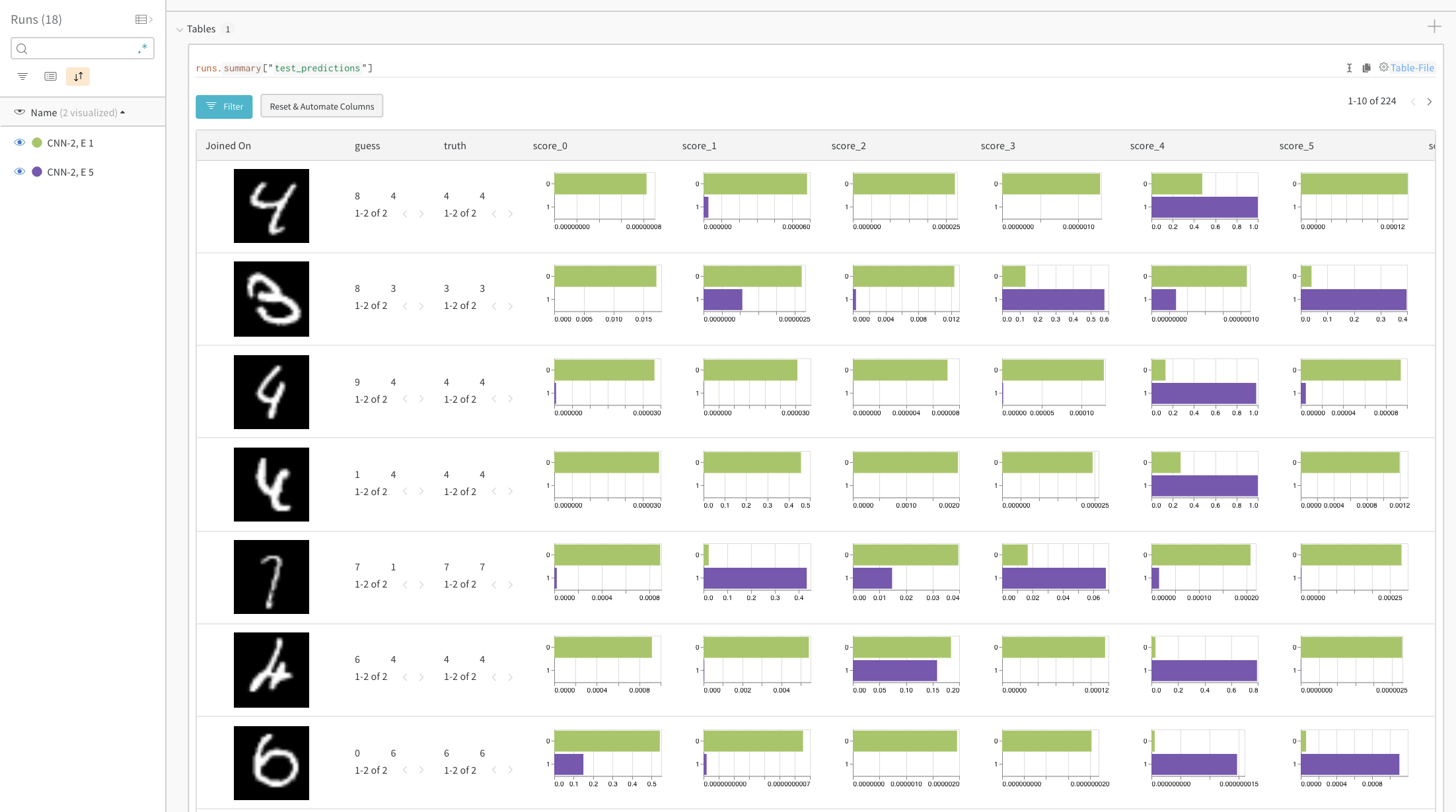
def log_image_table(images, predicted, labels, probs):
    "Log a wandb.Table with (img, pred, target, scores)"
    # 🐝 Create a wandb Table to log images, labels and predictions to
    table = wandb.Table(columns=["image", "pred", "target"]+[f"score_{i}" for i in range(10)])
    for img, pred, targ, prob in zip(images.to("cpu"), predicted.to("cpu"), labels.to("cpu"), probs.to("cpu")):
        table.add_data(wandb.Image(img[0].numpy()*255), pred, targ, *prob.numpy())
    wandb.log({"predictions_table":table}, commit=False)

Train Your Model

# Launch 5 experiments, trying different dropout rates
for _ in range(5):
    # 🐝 initialise a wandb run
    wandb.init(
        project="pytorch-intro",
        config={
            "epochs": 10,
            "batch_size": 128,
            "lr": 1e-3,
            "dropout": random.uniform(0.01, 0.80),
            })
    
    # Copy your config 
    config = wandb.config

    # Get the data
    train_dl = get_dataloader(is_train=True, batch_size=config.batch_size)
    valid_dl = get_dataloader(is_train=False, batch_size=2*config.batch_size)
    n_steps_per_epoch = math.ceil(len(train_dl.dataset) / config.batch_size)
    
    # A simple MLP model
    model = get_model(config.dropout)

    # Make the loss and optimizer
    loss_func = nn.CrossEntropyLoss()
    optimizer = torch.optim.Adam(model.parameters(), lr=config.lr)

   # Training
    example_ct = 0
    step_ct = 0
    for epoch in range(config.epochs):
        model.train()
        for step, (images, labels) in enumerate(train_dl):
            images, labels = images.to(device), labels.to(device)

            outputs = model(images)
            train_loss = loss_func(outputs, labels)
            optimizer.zero_grad()
            train_loss.backward()
            optimizer.step()
            
            example_ct += len(images)
            metrics = {"train/train_loss": train_loss, 
                       "train/epoch": (step + 1 + (n_steps_per_epoch * epoch)) / n_steps_per_epoch, 
                       "train/example_ct": example_ct}
            
            if step + 1 < n_steps_per_epoch:
                # 🐝 Log train metrics to wandb 
                wandb.log(metrics)
                
            step_ct += 1

        val_loss, accuracy = validate_model(model, valid_dl, loss_func, log_images=(epoch==(config.epochs-1)))

        # 🐝 Log train and validation metrics to wandb
        val_metrics = {"val/val_loss": val_loss, 
                       "val/val_accuracy": accuracy}
        wandb.log({**metrics, **val_metrics})
        
        print(f"Train Loss: {train_loss:.3f}, Valid Loss: {val_loss:3f}, Accuracy: {accuracy:.2f}")

    # If you had a test set, this is how you could log it as a Summary metric
    wandb.summary['test_accuracy'] = 0.8

    # 🐝 Close your wandb run 
    wandb.finish()

您现在已经使用 wandb 训练了您的第一个模型！ 👆 单击上面的 wandb 链接查看您的指标

Try W&B Alerts

W&B Alerts 允许您将从 Python 代码触发的警报发送到您的 Slack 或电子邮件。第一次发送 Slack 或电子邮件警报时，需要执行 2 个步骤，这些警报由您的代码触发：

1) 在你的 W&B User Settings 开启警报

2) 添加 wandb.alert() 到你的代码:

wandb.alert(
    title="Low accuracy", 
    text=f"Accuracy is below the acceptable threshold"
)

请参阅下面的最小示例以了解如何使用 wandb.alert，您可以在此处找到 W&B Alerts的完整文档

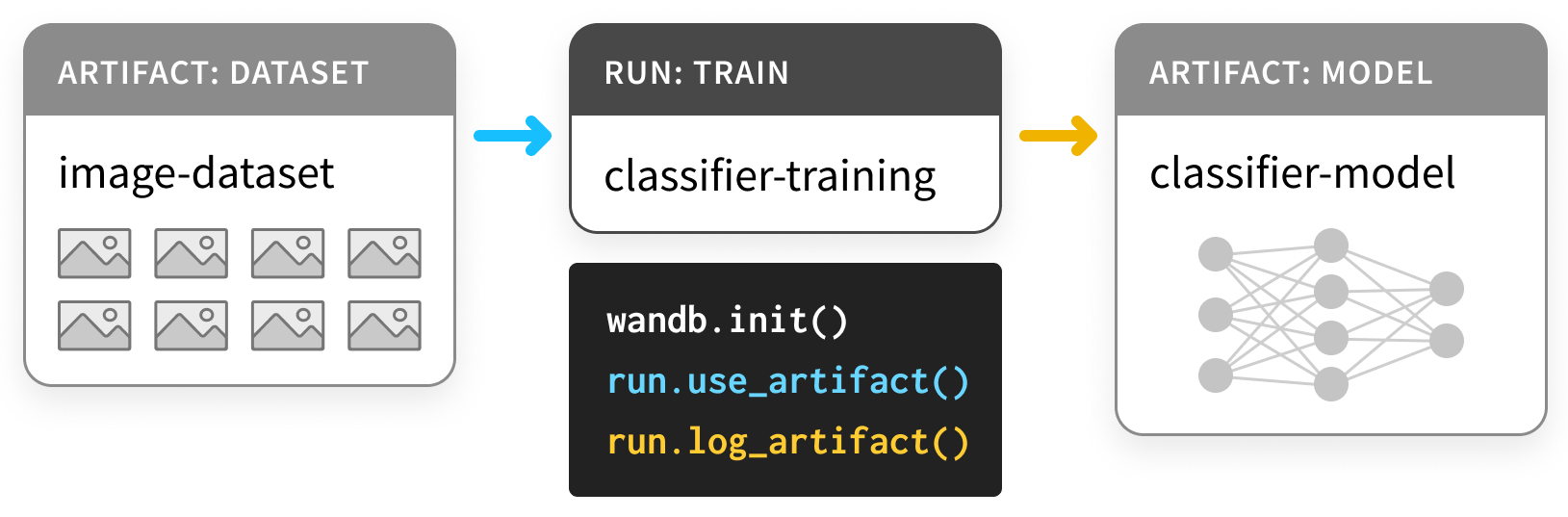
# Start a wandb run
wandb.init(project="pytorch-intro")

# Simulating a model training loop
acc_threshold = 0.3
for training_step in range(1000):

    # Generate a random number for accuracy
    accuracy = round(random.random() + random.random(), 3)
    print(f'Accuracy is: {accuracy}, {acc_threshold}')
    
    # 🐝 Log accuracy to wandb
    wandb.log({"Accuracy": accuracy})

    # 🔔 If the accuracy is below the threshold, fire a W&B Alert and stop the run
    if accuracy <= acc_threshold:
        # 🐝 Send the wandb Alert
        wandb.alert(
            title='Low Accuracy',
            text=f'Accuracy {accuracy} at step {training_step} is below the acceptable theshold, {acc_threshold}',
        )
        print('Alert triggered')
        break

# Mark the run as finished (useful in Jupyter notebooks)
wandb.finish()

Visualize predictions

这包括如何在训练过程中使用 PyTorch 对 MNIST 数据进行跟踪、可视化和比较模型预测。

你将学到如何：

1. 在模型训练或评估期间将指标、图像、文本等记录到 wandb.Table()
2. 查看、排序、筛选、分组、加入、交互式查询和探索这些表
3. 比较模型预测或结果：动态地跨越特定图像、超参数/模型版本或时间步长。

Examples

Compare predicted scores for specific images

实例：比较 1 和 5 个训练周期后的预测

1 epoch vs 5 epochs of training

直方图比较了两个模型之间的每类分数。每个直方图中顶部的绿色条代表模型“CNN-2, 1 epoch”（id 0），它只训练了 1 个 epoch。底部的紫色条代表模型“CNN-2, 5 epochs” (id 1)，它训练了 5 个 epochs。图像被过滤到模型不一致的情况。例如，在第一行中，“4”在 1 个时期后在所有可能的数字中获得高分，但在 5 个时期后，它在正确标签上得分最高，而在其余部分得分非常低。

Focus on top errors over time

实例 →

查看完整测试数据的不正确预测（过滤 "guess" != "truth" 的行）。请注意，在 1 个训练时期后有 229 个错误猜测，但在 5 个时期后只有 98 个。

side by side, 1 vs 5 epochs of training

Compare model performance and find patterns

查看实例中的完整详细信息 →

过滤出正确答案，然后按猜测分组，以查看错误分类图像的示例和真实标签的基本分布——并排显示两个模型。具有 2X layer sizes 和学习率的模型变体在左侧，基线在右侧。请注意，对于每个猜测的类，基线都会犯更多的错误。

grouped errors for baseline vs double variant

Sign up or login

Sign up or login W&B 以在浏览器中查看您的实验并与之互动。

在此示例中，我们使用 Google Colab 作为方便的托管环境，但您可以从任何地方运行自己的训练脚本，并使用 W&B 的实验跟踪工具可视化指标。

!pip install wandb -qqq

登录您的帐户

import wandb
wandb.login()

WANDB_PROJECT = "mnist-viz"

0. Setup

安装依赖项，下载 MNIST，并使用 PyTorch 创建训练和测试数据集。

import torch
import torch.nn as nn
import torchvision
import torchvision.transforms as T 
import torch.nn.functional as F


device = "cuda:0" if torch.cuda.is_available() else "cpu"

# create train and test dataloaders
def get_dataloader(is_train, batch_size, slice=5):
    "Get a training dataloader"
    ds = torchvision.datasets.MNIST(root=".", train=is_train, transform=T.ToTensor(), download=True)
    loader = torch.utils.data.DataLoader(dataset=ds, 
                                         batch_size=batch_size, 
                                         shuffle=True if is_train else False, 
                                         pin_memory=True, num_workers=2)
    return loader

1. Define the model and training schedule

• 设置要运行的纪元数，其中每个纪元包含一个训练步骤和一个验证（测试）步骤。 （可选）配置每个测试步骤要记录的数据量。这里要可视化的批次数和每批次的图像数设置得较低，以简化演示。
• 定义一个简单的卷积神经网络（遵循 pytorch-tutorial 代码）。
• 使用 PyTorch 加载训练集和测试集

# Number of epochs to run
# Each epoch includes a training step and a test step, so this sets
# the number of tables of test predictions to log
EPOCHS = 1

# Number of batches to log from the test data for each test step
# (default set low to simplify demo)
NUM_BATCHES_TO_LOG = 10 #79

# Number of images to log per test batch
# (default set low to simplify demo)
NUM_IMAGES_PER_BATCH = 32 #128

# training configuration and hyperparameters
NUM_CLASSES = 10
BATCH_SIZE = 32
LEARNING_RATE = 0.001
L1_SIZE = 32
L2_SIZE = 64
# changing this may require changing the shape of adjacent layers
CONV_KERNEL_SIZE = 5

# define a two-layer convolutional neural network
class ConvNet(nn.Module):
    def __init__(self, num_classes=10):
        super(ConvNet, self).__init__()
        self.layer1 = nn.Sequential(
            nn.Conv2d(1, L1_SIZE, CONV_KERNEL_SIZE, stride=1, padding=2),
            nn.BatchNorm2d(L1_SIZE),
            nn.ReLU(),
            nn.MaxPool2d(kernel_size=2, stride=2))
        self.layer2 = nn.Sequential(
            nn.Conv2d(L1_SIZE, L2_SIZE, CONV_KERNEL_SIZE, stride=1, padding=2),
            nn.BatchNorm2d(L2_SIZE),
            nn.ReLU(),
            nn.MaxPool2d(kernel_size=2, stride=2))
        self.fc = nn.Linear(7*7*L2_SIZE, NUM_CLASSES)
        self.softmax = nn.Softmax(NUM_CLASSES)

    def forward(self, x):
        # uncomment to see the shape of a given layer:
        #print("x: ", x.size())
        out = self.layer1(x)
        out = self.layer2(out)
        out = out.reshape(out.size(0), -1)
        out = self.fc(out)
        return out

train_loader = get_dataloader(is_train=True, batch_size=BATCH_SIZE)
test_loader = get_dataloader(is_train=False, batch_size=2*BATCH_SIZE)

device = torch.device("cuda:0" if torch.cuda.is_available() else "cpu")

2. Run training and log test predictions

对于每个时期，运行一个训练步骤和一个测试步骤。对于每个测试步骤，创建一个 wandb.Table() 来存储测试预测。这些可以在您的浏览器中进行可视化、动态查询和并排比较。

# ✨ W&B: Initialize a new run to track this model's training
wandb.init(project="table-quickstart")

# ✨ W&B: Log hyperparameters using config
cfg = wandb.config
cfg.update({"epochs" : EPOCHS, "batch_size": BATCH_SIZE, "lr" : LEARNING_RATE,
            "l1_size" : L1_SIZE, "l2_size": L2_SIZE,
            "conv_kernel" : CONV_KERNEL_SIZE,
            "img_count" : min(10000, NUM_IMAGES_PER_BATCH*NUM_BATCHES_TO_LOG)})

# define model, loss, and optimizer
model = ConvNet(NUM_CLASSES).to(device)
criterion = nn.CrossEntropyLoss()
optimizer = torch.optim.Adam(model.parameters(), lr=LEARNING_RATE)

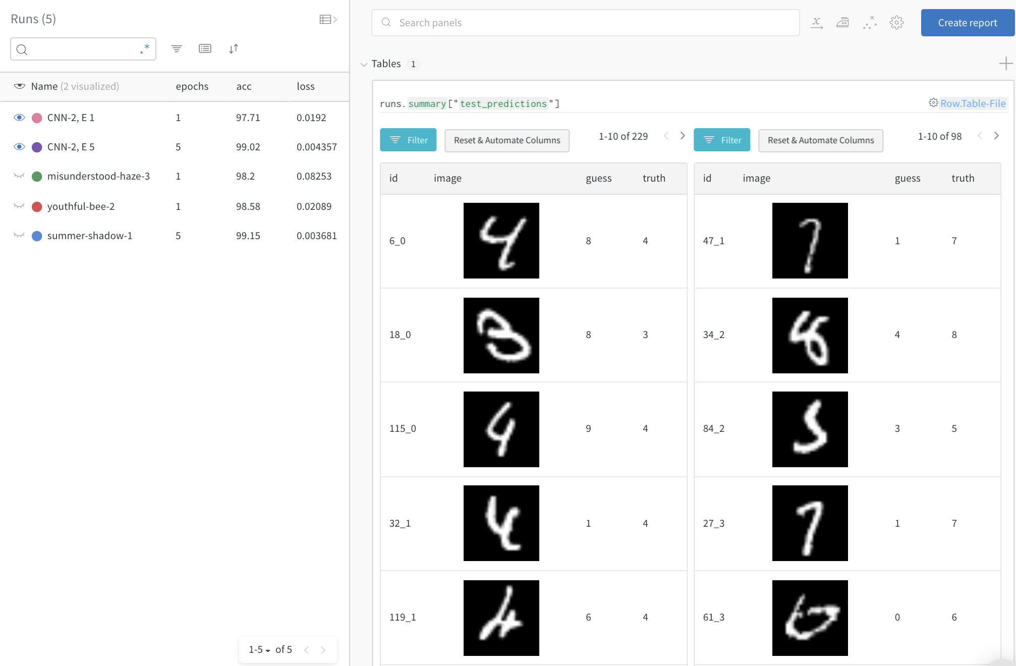
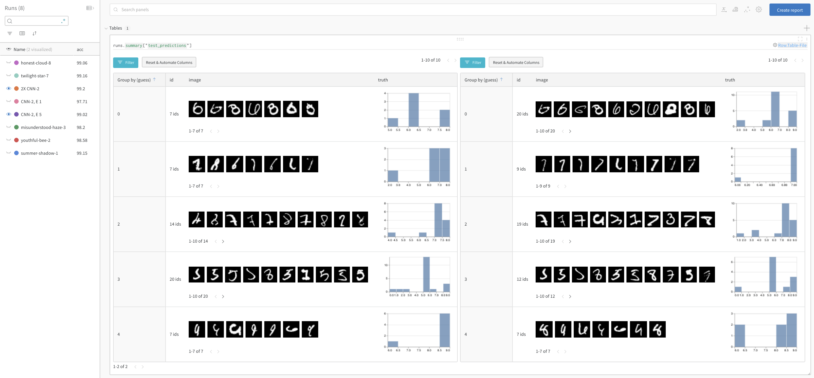
# convenience funtion to log predictions for a batch of test images
def log_test_predictions(images, labels, outputs, predicted, test_table, log_counter):
  # obtain confidence scores for all classes
  scores = F.softmax(outputs.data, dim=1)
  log_scores = scores.cpu().numpy()
  log_images = images.cpu().numpy()
  log_labels = labels.cpu().numpy()
  log_preds = predicted.cpu().numpy()
  # adding ids based on the order of the images
  _id = 0
  for i, l, p, s in zip(log_images, log_labels, log_preds, log_scores):
    # add required info to data table:
    # id, image pixels, model's guess, true label, scores for all classes
    img_id = str(_id) + "_" + str(log_counter)
    test_table.add_data(img_id, wandb.Image(i), p, l, *s)
    _id += 1
    if _id == NUM_IMAGES_PER_BATCH:
      break

# train the model
total_step = len(train_loader)
for epoch in range(EPOCHS):
    # training step
    for i, (images, labels) in enumerate(train_loader):
        images = images.to(device)
        labels = labels.to(device)
        # forward pass
        outputs = model(images)
        loss = criterion(outputs, labels)
        # backward and optimize
        optimizer.zero_grad()
        loss.backward()
        optimizer.step()
  
        # ✨ W&B: Log loss over training steps, visualized in the UI live
        wandb.log({"loss" : loss})
        if (i+1) % 100 == 0:
            print ('Epoch [{}/{}], Step [{}/{}], Loss: {:.4f}'
                .format(epoch+1, EPOCHS, i+1, total_step, loss.item()))
            

    # ✨ W&B: Create a Table to store predictions for each test step
    columns=["id", "image", "guess", "truth"]
    for digit in range(10):
      columns.append("score_" + str(digit))
    test_table = wandb.Table(columns=columns)

    # test the model
    model.eval()
    log_counter = 0
    with torch.no_grad():
        correct = 0
        total = 0
        for images, labels in test_loader:
            images = images.to(device)
            labels = labels.to(device)
            outputs = model(images)
            _, predicted = torch.max(outputs.data, 1)
            if log_counter < NUM_BATCHES_TO_LOG:
              log_test_predictions(images, labels, outputs, predicted, test_table, log_counter)
              log_counter += 1
            total += labels.size(0)
            correct += (predicted == labels).sum().item()

        acc = 100 * correct / total
        # ✨ W&B: Log accuracy across training epochs, to visualize in the UI
        wandb.log({"epoch" : epoch, "acc" : acc})
        print('Test Accuracy of the model on the 10000 test images: {} %'.format(acc))

    # ✨ W&B: Log predictions table to wandb
    wandb.log({"test_predictions" : test_table})

# ✨ W&B: Mark the run as complete (useful for multi-cell notebook)
wandb.finish()

Tune hyperparameters

在此处试用 Colab Notebook →

在高维超参数空间中搜索以找到性能最高的模型可能会很快变得笨拙。超参数扫描提供了一种有组织且高效的方式来进行模型大逃杀并选择最准确的模型。他们通过自动搜索超参数值的组合（例如 learning rate, batch size, number of hidden layers, optimizer type）来找到最佳值来实现这一点。

在本教程中，我们将了解如何使用 Weights & Biases 通过 3 个简单步骤运行复杂的超参数扫描。

Follow along with a video tutorial!

tune hyperparameters

Setup

首先安装实验跟踪库并设置您的免费 W&B 帐户：

1. 使用 pip install 安装
2. import Python 所需依赖
3. .login() 这样您就可以将指标记录到您的项目中

如果您以前从未使用过 Weights & Biases，登录电话会给您一个注册帐户的链接。 W&B 可免费用于个人和学术项目！

!pip install wandb -Uq

import wandb

wandb.login()

Step 1️⃣. Define the Sweep

从根本上说，Sweep 将尝试一堆超参数值的策略与评估它们的代码结合在一起。您只需要以配置的形式定义您的策略。

当您像这样在笔记本中设置 Sweep 时，该配置对象是一个嵌套字典。当您通过命令行运行 Sweep 时，配置对象是一个 YAML file。

让我们一起了解 Sweep 配置的定义。我们会慢慢来，这样我们就有机会解释每个组件。在典型的 Sweep 管道中，此步骤将在单个分配中完成。

Pick a method

我们需要定义的第一件事是选择新参数值的 method。

我们提供以下搜索 methods：

• grid Search – 迭代超参数值的每个组合。非常有效，但计算量大。
• random Search – 根据提供的 distribution 随机选择每个新组合。出乎意料的有效！
• bayesian Search – 创建一个度量分数作为超参数函数的概率模型，并选择具有提高度量的高概率的参数。适用于少量连续参数但扩展性差。

random 方法：

sweep_config = {
    'method': 'random'
    }

对于 bayesian Sweeps，您还需要告诉我们一些关于您的 metric 的信息。我们需要知道它的名称，以便我们可以在模型输出中找到它，我们需要知道您的目标是最小化它（例如，如果它是 squared error）还是最大化它（例如，如果它是 accuracy）。

metric = {
    'name': 'loss',
    'goal': 'minimize'   
    }

sweep_config['metric'] = metric

如果您没有运行 bayesian Sweep，则不必这样做，但无论如何将其包含在您的 sweep_config 中并不是一个坏主意，以防您以后改变主意。记录这样的事情也是很好的再现性实践，以防万一您或其他人在 6 个月或 6 年后回到您的 Sweep 并且不知道 val_G_batch 应该是高还是低。

Name the hyperparameters

一旦您选择了一种 method 来尝试超参数的新值，您需要定义这些 parameters是什么

大多数时候，这一步很简单：您只需为 parameter 命名并指定参数的合法 values 列表。

例如，当我们为我们的网络选择 optimizer 时，只有有限数量的选项。在这里，我们坚持使用两个最受欢迎的选择，adam 和 sgd。即使对于具有潜在无限选项的超参数，通常也只尝试几个选择 values 才有意义，就像我们在此处对隐藏层 layer_size 和 dropout 所做的那样。

parameters_dict = {
    'optimizer': {
        'values': ['adam', 'sgd']
        },
    'fc_layer_size': {
        'values': [128, 256, 512]
        },
    'dropout': {
          'values': [0.3, 0.4, 0.5]
        },
    }

sweep_config['parameters'] = parameters_dict

通常情况下，有些超参数我们不想在此 Sweep 中改变，但我们仍希望在我们的 sweep_config 中设置它们。

在那种情况下，我们直接设置 value：

parameters_dict.update({
    'epochs': {
        'value': 1}
    })

对于 grid 搜索，这就是您所需要的。

对于 random 搜索，参数的所有 values 在给定运行中被选择的可能性相同。

如果这样做不行，您可以改为指定命名 distribution 及其参数，例如 normal 分布的均值 mu 和标准差 sigma。

在此处查看有关如何设置随机变量分布的更多信息。

parameters_dict.update({
    'learning_rate': {
        # a flat distribution between 0 and 0.1
        'distribution': 'uniform',
        'min': 0,
        'max': 0.1
      },
    'batch_size': {
        # integers between 32 and 256
        # with evenly-distributed logarithms 
        'distribution': 'q_log_uniform_values',
        'q': 8,
        'min': 32,
        'max': 256,
      }
    })

当我们完成后，sweep_config 是一个嵌套的字典，它准确地指定了我们有兴趣尝试哪些 parameters 以及我们将使用什么 method 来尝试它们。

import pprint

pprint.pprint(sweep_config)

但这不是所有的配置选项！

例如，我们还提供了使用 HyperBand 调度算法 early_terminate 运行的选项。在这里查看更多。

您可以在此处找到所有配置选项的列表，并在此处找到大量 YAML 格式的示例。

Step 2️⃣. Initialize the Sweep

一旦您定义了搜索策略，就该设置一些东西来实现它了。

负责我们 Sweep 的 clockwork taskmaster 被称为 Sweep Controller。每次运行完成时，它将发出一组新的指令来描述要执行的新运行。这些指令由实际执行运行的 agents 获取。

在典型的 Sweep 中，Controller 位于我们的机器上，而完成运行的代理位于您的机器上，如下图所示。这种分工使得只需添加更多机器来运行代理就可以非常容易地扩展 Sweeps！

sweeps-diagram

我们可以通过使用适当的 sweep_config 和 project 名称调用 wandb.sweep 来结束 Sweep Controller。

此函数返回一个 sweep_id，我们稍后将使用它来将 agents 分配给此 Controller。

旁注：在命令行上，此功能被替换为

wandb sweep config.yaml

了解更多关于在命令行中使用 Sweeps ➡

sweep_id = wandb.sweep(sweep_config, project="pytorch-sweeps-demo")

Step 3️⃣. Run the Sweep agent

Define Your Training Procedure

在我们实际执行 sweep 之前，我们需要定义使用这些值的训练过程。

在下面的函数中，我们在 PyTorch 中定义了一个简单的全连接神经网络，并添加了以下 wandb 工具来记录模型指标、可视化性能和输出并跟踪我们的实验：

• wandb.init() – 初始化新的 W&B 运行。每次运行都是训练功能的一次执行。
• wandb.config – 将所有超参数保存在配置对象中，以便记录它们。在此处阅读有关如何使用 wandb.config 的更多信息。
• wandb.log() – 将模型行为记录到 W&B。在这里，我们只记录性能；有关可以使用 wandb.log 记录的所有其他富媒体，请参阅此 Colab。

有关使用 PyTorch 检测 W&B 的更多详细信息，请参阅此 Colab。

import torch
import torch.optim as optim
import torch.nn.functional as F
import torch.nn as nn
from torchvision import datasets, transforms

device = torch.device("cuda" if torch.cuda.is_available() else "cpu")

def train(config=None):
    # Initialize a new wandb run
    with wandb.init(config=config):
        # If called by wandb.agent, as below,
        # this config will be set by Sweep Controller
        config = wandb.config

        loader = build_dataset(config.batch_size)
        network = build_network(config.fc_layer_size, config.dropout)
        optimizer = build_optimizer(network, config.optimizer, config.learning_rate)

        for epoch in range(config.epochs):
            avg_loss = train_epoch(network, loader, optimizer)
            wandb.log({"loss": avg_loss, "epoch": epoch})           

这个单元格定义了我们训练过程的四个部分：build_dataset, build_network, build_optimizer 和train_epoch.

所有这些都是基本 PyTorch 管道的标准部分，它们的实现不受使用 W&B 的影响，因此我们不会对它们发表评论。

def build_dataset(batch_size):
   
    transform = transforms.Compose(
        [transforms.ToTensor(),
         transforms.Normalize((0.1307,), (0.3081,))])
    # download MNIST training dataset
    dataset = datasets.MNIST(".", train=True, download=True,
                             transform=transform)
    sub_dataset = torch.utils.data.Subset(
        dataset, indices=range(0, len(dataset), 5))
    loader = torch.utils.data.DataLoader(sub_dataset, batch_size=batch_size)

    return loader


def build_network(fc_layer_size, dropout):
    network = nn.Sequential(  # fully-connected, single hidden layer
        nn.Flatten(),
        nn.Linear(784, fc_layer_size), nn.ReLU(),
        nn.Dropout(dropout),
        nn.Linear(fc_layer_size, 10),
        nn.LogSoftmax(dim=1))

    return network.to(device)
        

def build_optimizer(network, optimizer, learning_rate):
    if optimizer == "sgd":
        optimizer = optim.SGD(network.parameters(),
                              lr=learning_rate, momentum=0.9)
    elif optimizer == "adam":
        optimizer = optim.Adam(network.parameters(),
                               lr=learning_rate)
    return optimizer


def train_epoch(network, loader, optimizer):
    cumu_loss = 0
    for _, (data, target) in enumerate(loader):
        data, target = data.to(device), target.to(device)
        optimizer.zero_grad()

        # ➡ Forward pass
        loss = F.nll_loss(network(data), target)
        cumu_loss += loss.item()

        # ⬅ Backward pass + weight update
        loss.backward()
        optimizer.step()

        wandb.log({"batch loss": loss.item()})

    return cumu_loss / len(loader)

现在，我们准备开始 sweeping 了！

Sweep Controllers，就像我们通过运行 wandb.sweep 制作的控制器一样，坐等有人要求他们提供 config来试用。

某人是 agent，他们是用 wandb.agent 创建的。要开始，agent 只需要知道

1. 它是 (sweep_id) 的一部分
2. 它应该运行哪个函数（这里是 train）
3. （可选）有多少配置要求控制器（count）

仅供参考，您可以在不同的计算资源上启动具有相同 sweep_id 的多个 agent，Controller 将确保它们根据 sweep_config 中制定的策略协同工作。这使得在尽可能多的节点上扩展 Sweeps 变得轻而易举！

旁注：在命令行上，此功能被替换为

wandb agent sweep_id

了解更多关于在命令行中使用 Sweeps ➡

下面的单元格将启动一个运行 train 5 次的 agent，使用 Sweep Controller 返回的随机生成的超参数值。执行时间不到 5 分钟。

wandb.agent(sweep_id, train, count=5)

Visualize Sweep Results

Parallel Coordinates Plot

此图将超参数值映射到模型指标。它对于磨练导致最佳模型性能的超参数组合很有用。

hyperparameters map to metrics

Hyperparameter Importance Plot

超参数重要性图表明哪些超参数是指标的最佳预测因子。我们报告特征重要性（来自随机森林模型）和相关性（隐式线性模型）。

parameter importance

这些可视化可以通过磨练最重要的参数（和值范围）来帮助您节省运行昂贵的超参数优化的时间和资源，因此值得进一步探索。

Get your hands dirty with sweeps

我们创建了一个简单的训练脚本和一些 sweep configs 风格供您使用。我们强烈建议您尝试一下。

该存储库还提供了一些示例，可帮助您尝试更高级的 sweep 功能，例如 Bayesian Hyperband 和 Hyperopt。

Track models and datasets

在此处试用 Colab Notebook →

在此笔记本中，我们将向您展示如何使用 W&B Artifacts 跟踪您的 ML 实验管道。

Follow along with a video tutorial!

What are Artifacts and Why Should I Care?

“artifact”，如希腊双耳瓶🏺，是一个生产的对象——一个过程的输出。在 ML 中，最重要的工件是 datasets 和 models。

而且，就像 Cross of Coronado 一样，这些重要的文物属于博物馆！也就是说，应该对它们进行分类和组织，以便您、您的团队和整个 ML 社区可以向它们学习。毕竟，那些不跟踪训练的人注定要重蹈覆辙。

使用我们的 Artifacts API，您可以将 Artifacts 记录为 W&B Runs 的输出，或使用 Artifacts 作为 Runs 的输入，如此图所示，其中训练运行接受数据集并生成模型。

simple artifact diagram

由于一次运行可以使用另一次的输出作为输入，因此 Artifacts 和 Runs 一起形成了一个有向图——实际上是一个二分 DAG！ -- 带有 Artifacts 和 Runs 的节点，以及将 Runs 连接到它们消耗或生产的 Artifacts 的箭头。

0️⃣ Install and Import

Artifacts 是我们 Python 库的一部分，从 0.9.2 版开始。

与 ML Python 堆栈的大多数部分一样，它可以通过 pip 获得。

# Compatible with wandb version 0.9.2+
!pip install wandb -qqq
!apt install tree

import os
import wandb

1️⃣ Log a Dataset

首先，让我们定义一些 Artifacts。

此示例基于此 PyTorch "Basic MNIST Example"，但可以在 TensorFlow、任何其他框架或纯 Python 中轻松完成。

我们从 Datasets 开始：

• 一个 training set，用于选择参数，
• 一个 validation set，用于选择超参数，
• 一个 testing set，用于评估最终模型

下面的第一个单元格定义了这三个数据集。

import random 

import torch
import torchvision
from torch.utils.data import TensorDataset
from tqdm.auto import tqdm

# Ensure deterministic behavior
torch.backends.cudnn.deterministic = True
random.seed(0)
torch.manual_seed(0)
torch.cuda.manual_seed_all(0)

# Device configuration
device = torch.device("cuda:0" if torch.cuda.is_available() else "cpu")

# Data parameters
num_classes = 10
input_shape = (1, 28, 28)

# drop slow mirror from list of MNIST mirrors
torchvision.datasets.MNIST.mirrors = [mirror for mirror in torchvision.datasets.MNIST.mirrors
                                      if not mirror.startswith("http://yann.lecun.com")]

def load(train_size=50_000):
    """
    # Load the data
    """

    # the data, split between train and test sets
    train = torchvision.datasets.MNIST("./", train=True, download=True)
    test = torchvision.datasets.MNIST("./", train=False, download=True)
    (x_train, y_train), (x_test, y_test) = (train.data, train.targets), (test.data, test.targets)

    # split off a validation set for hyperparameter tuning
    x_train, x_val = x_train[:train_size], x_train[train_size:]
    y_train, y_val = y_train[:train_size], y_train[train_size:]

    training_set = TensorDataset(x_train, y_train)
    validation_set = TensorDataset(x_val, y_val)
    test_set = TensorDataset(x_test, y_test)

    datasets = [training_set, validation_set, test_set]

    return datasets

这建立了一个模式，我们将在这个例子中看到重复：将数据记录为工件的代码包裹在生成该数据的代码周围。在这种情况下，用于 loading 数据的代码与用于 load_and_logging 数据的代码分开。

这是很好的做法！

为了将这些数据集记录为工件，我们只需要

1. 使用 wandb.init 创建 Run，(L4)
2. 为数据集 (L10) 创建一个 Artifact，以及
3. 保存并记录相关 files（L20、L23）。

查看下面代码单元的示例，然后展开后面的部分以了解更多详细信息。

def load_and_log():

    # 🚀 start a run, with a type to label it and a project it can call home
    with wandb.init(project="artifacts-example", job_type="load-data") as run:
        
        datasets = load()  # separate code for loading the datasets
        names = ["training", "validation", "test"]

        # 🏺 create our Artifact
        raw_data = wandb.Artifact(
            "mnist-raw", type="dataset",
            description="Raw MNIST dataset, split into train/val/test",
            metadata={"source": "torchvision.datasets.MNIST",
                      "sizes": [len(dataset) for dataset in datasets]})

        for name, data in zip(names, datasets):
            # 🐣 Store a new file in the artifact, and write something into its contents.
            with raw_data.new_file(name + ".pt", mode="wb") as file:
                x, y = data.tensors
                torch.save((x, y), file)

        # ✍️ Save the artifact to W&B.
        run.log_artifact(raw_data)

load_and_log()

🚀 wandb.init

当我们制作将要产生 Artifacts 的 Run时，我们需要说明它属于哪个 project。

根据您的工作流程，项目可能大到 car-that-drives-itself，也可能小到 iterative-architecture-experiment-117。

Depending on your workflow, a project might be as big as car-that-drives-itself or as small as iterative-architecture-experiment-117.

👍规则：如果可以，请将所有共享 Artifacts 的 Runs 保留在一个项目中。这使事情变得简单，但不要担心 Artifacts 可以跨项目移植！

为了帮助跟踪您可能运行的所有不同类型的作业，在进行 Runs 时提供 job_type 很有用。这可以使您的 Artifacts 图表保持整洁。

👍规则：job_type 应该是描述性的，并且对应于你的管道的单个步骤。在这里，我们将 loading 数据与 preprocessing 数据分开。

🏺 wandb.Artifact

要将某物记录为 Artifact，我们必须首先创建一个 Artifact 对象。

每个 Artifact 都有一个 name——这是第一个参数设置的名称。

👍的规则：name 应该是描述性的，但易于记忆和输入——我们喜欢使用连字符分隔的名称，并与代码中的变量名相对应。

它也有一个 type。就像 Runs 的 job_types 一样，它用于组织 Runs 和 Artifacts 的图表。

👍的规则：type 应该简单：比 mnist-data-YYYYMMDD 更像 dataset 或 model。

您还可以附加 description 和一些 metadata，作为字典。metadata 只需要可序列化为 JSON。

👍规则：metadata应尽可能具有描述性。

🐣 artifact.new_file and ✍️ run.log_artifact

一旦我们创建了一个 Artifact 对象，我们需要向它添加文件。

您没看错：带有 s 的 files。Artifacts 的结构类似于目录，包含文件和子目录。

👍规则：只要有必要，将 Artifact 的内容拆分为多个文件。如果需要扩展，这将有所帮助！

我们使用 new_file 方法同时写入文件并将其附加到 Artifact。下面，我们将使用 add_file 方法，它将这两个步骤分开

添加完所有文件后，我们需要将 log_artifact 添加到 wandb.ai。

您会注意到一些 URL 出现在输出中，包括一个用于运行页面的 URL。您可以在此处查看 Run 结果，包括已记录的任何 Artifacts。

我们将在下面看到一些示例，这些示例可以更好地利用“运行”页面的其他组件。

2️⃣ Use a Logged Dataset Artifact

与博物馆中的 artifacts 不同，W&B 中的 Artifacts 旨在使用，而不仅仅是存储。

让我们看看它是什么样的。

下面的单元格定义了一个管道步骤，该步骤接收原始数据集并使用它来生成 preprocessed 数据集：normalized 和正确整形。

再次注意，我们从与 wandb 接口的代码中分离出了代码的主体，即 preprocess。

def preprocess(dataset, normalize=True, expand_dims=True):
    """
    ## Prepare the data
    """
    x, y = dataset.tensors

    if normalize:
        # Scale images to the [0, 1] range
        x = x.type(torch.float32) / 255

    if expand_dims:
        # Make sure images have shape (1, 28, 28)
        x = torch.unsqueeze(x, 1)
    
    return TensorDataset(x, y)

现在是使用 wandb.Artifact 日志记录这个 preprocess 步骤的代码。

请注意，下面的示例都 uses 了一个新的 Artifact，并将其 logs 下来，这与上一步相同。Artifacts 既是 Runs 的输入又是输出！

我们使用一个新的 job_type，preprocess-data，来明确这是一个不同于之前的 job。

def preprocess_and_log(steps):

    with wandb.init(project="artifacts-example", job_type="preprocess-data") as run:

        processed_data = wandb.Artifact(
            "mnist-preprocess", type="dataset",
            description="Preprocessed MNIST dataset",
            metadata=steps)
         
        # ✔️ declare which artifact we'll be using
        raw_data_artifact = run.use_artifact('mnist-raw:latest')

        # 📥 if need be, download the artifact
        raw_dataset = raw_data_artifact.download()
        
        for split in ["training", "validation", "test"]:
            raw_split = read(raw_dataset, split)
            processed_dataset = preprocess(raw_split, **steps)

            with processed_data.new_file(split + ".pt", mode="wb") as file:
                x, y = processed_dataset.tensors
                torch.save((x, y), file)

        run.log_artifact(processed_data)


def read(data_dir, split):
    filename = split + ".pt"
    x, y = torch.load(os.path.join(data_dir, filename))

    return TensorDataset(x, y)

这里要注意的一件事是预处理的 steps 作为 metadata 与 preprocessed_data 一起保存。

如果您想让您的实验可重现，捕获大量元数据是个好主意！

此外，即使我们的数据集是 "large artifact"，download 步骤也可以在不到一秒的时间内完成。

展开下面的 markdown 单元格以了解详细信息。

steps = {"normalize": True,
         "expand_dims": True}

preprocess_and_log(steps)

✔️ run.use_artifact

这些步骤比较简单。消费者只需要知道 Artifact 的name，再加上 bit more。

“bit more” 是您想要的 Artifact 的特定版本的 alias。

默认情况下，最后上传的版本被标记为latest。否则，您可以选择带有 v0/v1 等的旧版本，或者您可以提供自己的别名，例如 best 或 jit-script。就像 Docker Hub 标签一样，别名与名称用 : 分隔，所以我们想要的 Artifact 是 mnist-raw:latest。

👍规则：保持别名简短而甜美。当您想要满足某些属性的 Artifact 时，请使用自定义 aliases，如 latest 或 best

📥 artifact.download

现在，您可能正在担心 download 调用。如果我们再下载一份，内存的负担会不会加倍？

别担心，朋友。在我们实际下载任何东西之前，我们会检查本地是否有正确的版本。使用和版本控制 git 和 torrenting 相同的技术：hashing。

随着 Artifacts 的创建和记录，工作目录中名为 artifacts 的文件夹将开始填充子目录，每个 Artifact一个。使用 !tree artifacts 检查其内容：

!tree artifacts

🌐 The Artifacts page on wandb.ai

现在我们已经记录并使用了一个 Artifact，让我们检查一下 Run 页面上的 Artifacts 选项卡。

从wandb 输出导航到运行页面 URL，然后从左侧边栏中选择“工件”选项卡（它是带有数据库图标的选项卡，看起来像三个冰球叠在一起）。

单击 "Input Artifacts" 表或 "Output Artifacts" 表中的一行，然后查看选项卡（"Overview", "Metadata"）以查看记录的有关 Artifact 的所有内容。

我们特别喜欢 "Graph View"。默认情况下，它显示一个图表，其中 Artifacts 的 types 和 Run 的 job_types 是两种类型的节点，箭头代表消费和生产。

3️⃣ Log a Model

这足以了解 Artifacts 的 API 如何工作，但让我们按照这个示例一直到管道的末尾，以便我们可以了解 Artifacts 如何改进您的 ML 工作流程。

这里的第一个单元格在 PyTorch 中构建了一个 DNN model——一个非常简单的 ConvNet。

我们将从初始化 model 开始，而不是训练它。这样，我们可以重复训练，同时保持其他一切不变。

from math import floor

import torch.nn as nn

class ConvNet(nn.Module):
    def __init__(self, hidden_layer_sizes=[32, 64],
                  kernel_sizes=[3],
                  activation="ReLU",
                  pool_sizes=[2],
                  dropout=0.5,
                  num_classes=num_classes,
                  input_shape=input_shape):
      
        super(ConvNet, self).__init__()

        self.layer1 = nn.Sequential(
              nn.Conv2d(in_channels=input_shape[0], out_channels=hidden_layer_sizes[0], kernel_size=kernel_sizes[0]),
              getattr(nn, activation)(),
              nn.MaxPool2d(kernel_size=pool_sizes[0])
        )
        self.layer2 = nn.Sequential(
              nn.Conv2d(in_channels=hidden_layer_sizes[0], out_channels=hidden_layer_sizes[-1], kernel_size=kernel_sizes[-1]),
              getattr(nn, activation)(),
              nn.MaxPool2d(kernel_size=pool_sizes[-1])
        )
        self.layer3 = nn.Sequential(
              nn.Flatten(),
              nn.Dropout(dropout)
        )

        fc_input_dims = floor((input_shape[1] - kernel_sizes[0] + 1) / pool_sizes[0]) # layer 1 output size
        fc_input_dims = floor((fc_input_dims - kernel_sizes[-1] + 1) / pool_sizes[-1]) # layer 2 output size
        fc_input_dims = fc_input_dims*fc_input_dims*hidden_layer_sizes[-1] # layer 3 output size

        self.fc = nn.Linear(fc_input_dims, num_classes)

    def forward(self, x):
        x = self.layer1(x)
        x = self.layer2(x)
        x = self.layer3(x)
        x = self.fc(x)
        return x

在这里，我们使用 W&B 来跟踪运行，因此使用 wandb.config 对象来存储所有超参数。

该 config 对象的 dictionary 版本是一个非常有用的 metadata，所以一定要包含它！

def build_model_and_log(config):
    with wandb.init(project="artifacts-example", job_type="initialize", config=config) as run:
        config = wandb.config
        
        model = ConvNet(**config)

        model_artifact = wandb.Artifact(
            "convnet", type="model",
            description="Simple AlexNet style CNN",
            metadata=dict(config))

        torch.save(model.state_dict(), "initialized_model.pth")
        # ➕ another way to add a file to an Artifact
        model_artifact.add_file("initialized_model.pth")

        wandb.save("initialized_model.pth")

        run.log_artifact(model_artifact)

model_config = {"hidden_layer_sizes": [32, 64],
                "kernel_sizes": [3],
                "activation": "ReLU",
                "pool_sizes": [2],
                "dropout": 0.5,
                "num_classes": 10}

build_model_and_log(model_config)

➕ artifact.add_file

与在数据集日志记录示例中同时编写 new_file 并将其添加到 Artifact 不同，我们还可以一步写入文件（此处为 torch.save），然后在另一步中将它们 add 到 Artifact。

👍规则：尽可能使用 new_file，以防止重复。

4️⃣ Use a Logged Model Artifact

就像我们可以在 dataset 上调用 use_artifact 一样，我们可以在我们的 initialized_model 上调用它以在另一个运行中使用它。

这一次，让我们 train model。

有关更多详细信息，请查看我们关于 instrumenting W&B with PyTorch 的 Colab。

import torch.nn.functional as F

def train(model, train_loader, valid_loader, config):
    optimizer = getattr(torch.optim, config.optimizer)(model.parameters())
    model.train()
    example_ct = 0
    for epoch in range(config.epochs):
        for batch_idx, (data, target) in enumerate(train_loader):
            data, target = data.to(device), target.to(device)
            optimizer.zero_grad()
            output = model(data)
            loss = F.cross_entropy(output, target)
            loss.backward()
            optimizer.step()

            example_ct += len(data)

            if batch_idx % config.batch_log_interval == 0:
                print('Train Epoch: {} [{}/{} ({:.0%})]\tLoss: {:.6f}'.format(
                    epoch, batch_idx * len(data), len(train_loader.dataset),
                    batch_idx / len(train_loader), loss.item()))
                
                train_log(loss, example_ct, epoch)

        # evaluate the model on the validation set at each epoch
        loss, accuracy = test(model, valid_loader)  
        test_log(loss, accuracy, example_ct, epoch)

    
def test(model, test_loader):
    model.eval()
    test_loss = 0
    correct = 0
    with torch.no_grad():
        for data, target in test_loader:
            data, target = data.to(device), target.to(device)
            output = model(data)
            test_loss += F.cross_entropy(output, target, reduction='sum')  # sum up batch loss
            pred = output.argmax(dim=1, keepdim=True)  # get the index of the max log-probability
            correct += pred.eq(target.view_as(pred)).sum()

    test_loss /= len(test_loader.dataset)

    accuracy = 100. * correct / len(test_loader.dataset)
    
    return test_loss, accuracy


def train_log(loss, example_ct, epoch):
    loss = float(loss)

    # where the magic happens
    wandb.log({"epoch": epoch, "train/loss": loss}, step=example_ct)
    print(f"Loss after " + str(example_ct).zfill(5) + f" examples: {loss:.3f}")
    

def test_log(loss, accuracy, example_ct, epoch):
    loss = float(loss)
    accuracy = float(accuracy)

    # where the magic happens
    wandb.log({"epoch": epoch, "validation/loss": loss, "validation/accuracy": accuracy}, step=example_ct)
    print(f"Loss/accuracy after " + str(example_ct).zfill(5) + f" examples: {loss:.3f}/{accuracy:.3f}")

这次我们将运行两个独立的 Artifact 生产 Runs。

一旦第一个完成 training model，第二个将通过评估其在 test_dataset 上的性能来使用 trained-model Artifact。

此外，我们将提取网络最混乱的 32 个示例——在这些示例中，categorical_crossentropy 最高。

这是诊断数据集和模型问题的好方法！

def evaluate(model, test_loader):
    """
    ## Evaluate the trained model
    """

    loss, accuracy = test(model, test_loader)
    highest_losses, hardest_examples, true_labels, predictions = get_hardest_k_examples(model, test_loader.dataset)

    return loss, accuracy, highest_losses, hardest_examples, true_labels, predictions

def get_hardest_k_examples(model, testing_set, k=32):
    model.eval()

    loader = DataLoader(testing_set, 1, shuffle=False)

    # get the losses and predictions for each item in the dataset
    losses = None
    predictions = None
    with torch.no_grad():
        for data, target in loader:
            data, target = data.to(device), target.to(device)
            output = model(data)
            loss = F.cross_entropy(output, target)
            pred = output.argmax(dim=1, keepdim=True)
            
            if losses is None:
                losses = loss.view((1, 1))
                predictions = pred
            else:
                losses = torch.cat((losses, loss.view((1, 1))), 0)
                predictions = torch.cat((predictions, pred), 0)

    argsort_loss = torch.argsort(losses, dim=0)

    highest_k_losses = losses[argsort_loss[-k:]]
    hardest_k_examples = testing_set[argsort_loss[-k:]][0]
    true_labels = testing_set[argsort_loss[-k:]][1]
    predicted_labels = predictions[argsort_loss[-k:]]

    return highest_k_losses, hardest_k_examples, true_labels, predicted_labels

这些日志记录功能不会添加任何新的 Artifact 功能，因此我们不会对其进行评论：我们只是在使用、下载和记录 Artifacts。

from torch.utils.data import DataLoader

def train_and_log(config):

    with wandb.init(project="artifacts-example", job_type="train", config=config) as run:
        config = wandb.config

        data = run.use_artifact('mnist-preprocess:latest')
        data_dir = data.download()

        training_dataset =  read(data_dir, "training")
        validation_dataset = read(data_dir, "validation")

        train_loader = DataLoader(training_dataset, batch_size=config.batch_size)
        validation_loader = DataLoader(validation_dataset, batch_size=config.batch_size)
        
        model_artifact = run.use_artifact("convnet:latest")
        model_dir = model_artifact.download()
        model_path = os.path.join(model_dir, "initialized_model.pth")
        model_config = model_artifact.metadata
        config.update(model_config)

        model = ConvNet(**model_config)
        model.load_state_dict(torch.load(model_path))
        model = model.to(device)
 
        train(model, train_loader, validation_loader, config)

        model_artifact = wandb.Artifact(
            "trained-model", type="model",
            description="Trained NN model",
            metadata=dict(model_config))

        torch.save(model.state_dict(), "trained_model.pth")
        model_artifact.add_file("trained_model.pth")
        wandb.save("trained_model.pth")

        run.log_artifact(model_artifact)

    return model

    
def evaluate_and_log(config=None):
    
    with wandb.init(project="artifacts-example", job_type="report", config=config) as run:
        data = run.use_artifact('mnist-preprocess:latest')
        data_dir = data.download()
        testing_set = read(data_dir, "test")

        test_loader = torch.utils.data.DataLoader(testing_set, batch_size=128, shuffle=False)

        model_artifact = run.use_artifact("trained-model:latest")
        model_dir = model_artifact.download()
        model_path = os.path.join(model_dir, "trained_model.pth")
        model_config = model_artifact.metadata

        model = ConvNet(**model_config)
        model.load_state_dict(torch.load(model_path))
        model.to(device)

        loss, accuracy, highest_losses, hardest_examples, true_labels, preds = evaluate(model, test_loader)

        run.summary.update({"loss": loss, "accuracy": accuracy})

        wandb.log({"high-loss-examples":
            [wandb.Image(hard_example, caption=str(int(pred)) + "," +  str(int(label)))
             for hard_example, pred, label in zip(hardest_examples, preds, true_labels)]})

train_config = {"batch_size": 128,
                "epochs": 5,
                "batch_log_interval": 25,
                "optimizer": "Adam"}

model = train_and_log(train_config)
evaluate_and_log()

🔁 The Graph View

请注意，我们更改了 Artifact 的 type：这些 Runs 使用的是模型，而不是数据集。在 Artifacts 页面的图形视图中，生产模型的 Runs 将与生成 datasets 的运行分开。

去看看吧！和以前一样，您需要前往 Run 页面，从左侧栏中选择 "Artifacts" 选项卡，选择一个 Artifact，然后单击 "Graph View" 选项卡。

💣 Exploded Graphs

您可能已经注意到标有“爆炸”的按钮。不要点击它，因为它会在 W&B 总部您不起眼的作者办公桌下引爆一枚小炸弹！

只是在开玩笑。它以更温和的方式“分解”图表：Artifacts 和 Runs 在单个实例级别而不是类型级别分离：节点不是 dataset 和 load-data，而是 dataset:mnist-raw:v1 和 load-data:sunny-smoke-1，等等。

这提供了对您的管道的全面洞察，记录的指标、元数据等都触手可及——您仅受限于您选择与我们一起记录的内容。